|
|
|
The FFT is ideally suited for homogeneous-type waveforms (waveforms that have the same structure throughout, or have a similar cyclic repetition) but need not be limited to this type. Before an FFT can be generated, the channel you wish to transform must be moved into display window one using the Variable Waveform Assignments function (e.g., type “1=5” if you wish to transform channel 5). After this is accomplished, scroll the display of the selected channel to center the area you wish to transform on the screen. The FFT can now be generated directly from either the Y-T or the X-Y display modes as follows:
![]() In
the Transform menu click on Windowed FFT….
In
the Transform menu click on Windowed FFT….
![]() Choose
Transform Windowed FFT… (ALT,
T, W).
Choose
Transform Windowed FFT… (ALT,
T, W).
This displays the FFT Window Type, Size, and Averaging dialog box as follows:
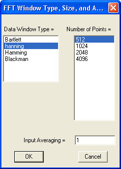
From this dialog box, you are able to select the type of FFT window that will be applied, the size of the FFT, and the input averaging factor.
The FFT algorithm supports four different types of windows that may be applied to minimize the effects of end-point distortion. These are Bartlett, hanning, Hamming, and Blackman windows. The characteristics of each window are described by the following figure:
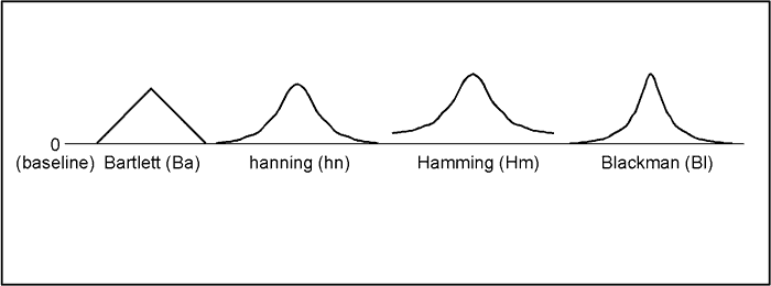
Each window has different characteristics that make one window better than another at separating spectral components near each other in frequency, or at isolating one spectral component that is much smaller than another, or whatever the task. The window that you use depends on your skill at manipulating the tradeoffs between the various windows and also on what you want to get out of the power spectrum or its inverse.
The FFT algorithm supports a number of different sized FFTs (size refers to the number of data points contained in the FFT). Because the FFT function uses a base 2 logarithm by definition, the range or length of the time series to be evaluated must contain a number of data points equal to a 2n number. This is why the FFT selections you see in the Number of Points list box are all a power of 2 (256, 512, 1024, etc.). The number of selections you see displayed in this list box will vary for any one data file depending on the factors that affect this power-of-2 limitation. These factors include the size of the data file, the width of the window that the WinDaq Waveform Browser program is running in on your monitor, the screen format (whether overlapped or non-overlapped), and whether or not the data file is compressed. The overall size of the data file determines whether or not the larger FFT options (such as 8192 and 16384) are displayed in the list box, while the size of the window that WinDaq Waveform Browser is running in and the screen format determines whether or not the smaller FFT options (such as 32, 64, or 128 points) are displayed. The minimum sized FFT that can be displayed in the list box is 32, and the maximum is 16384.
When the FFT algorithm is first initiated with an uncompressed waveform, the FFT selection highlighted in the Number of Points list box is the maximum power of 2 that will fit on the screen. For example, with a video standard of 1024 x 768, 1024 pixels of horizontal screen resolution are available for display. In this case, 1024 is a power of 2, so the 1024-point FFT selection will be highlighted in the Number of Points list box. When the OK command button is activated and the 1024-point FFT is performed, the data to be transformed is taken from the center of the screen in window 1. 512 data points in both directions from the center of the screen will be transformed. Similarly with a 2048 point FFT, 1024 data points in both directions are included in the FFT calculation, and so on with the other choices.
Note that you are not limited to only a 1024-point FFT. You can select a smaller or larger sized FFT from the list. So which size FFT is right for your waveform? That depends on what you want to see in the power spectrum and how much resolution you want. Beside calculation speed (which is negligible), the only difference between a 512-point transform and a 16384-point transform is resolution. A power spectrum always ranges from the dc level (0 Hz) to one-half the sample rate of the waveform being transformed, so the number of points in the transform defines the power spectrum resolution (a 512-point FFT would have 256 points in its power spectrum, a 1024-point FFT would have 512 points in its power spectrum, and so on). Suppose you wanted to see separate 20 and 21 Hz frequency components in the power spectrum of a complex waveform. A 512-point FFT might not show these individual components clearly since its entire power spectrum is only divided into 256 equally spaced points and the desired frequencies are so close together. However, if the transform contained more points, it would be able to devote more points to the definition of closely spaced frequency components. The more the number of points in a transform, the better the frequency resolution.
When you select an FFT from the list that is larger than the number of horizontal pixels your screen is capable of displaying, the waveform will automatically be compressed. This happens semi-transparently and requires no additional user input. The compression becomes obvious when the split screen display is exited (with the View, Exit/Enter Split command) and the normal Y-T waveform display is shown.
If you would like to perform a smaller FFT than what is shown on the list, you will have to reduce the amount of pixels your screen has available for display (the less you see, the less you FFT). This can be done primarily by horizontally shrinking or resizing the window that WinDaq Waveform Browser software is running in, and to a lesser degree by selecting an overlapped screen format. Refer to your Windows™ documentation for details on resizing the window border. Refer to Display Format Selection for details on selecting an overlapped screen format. For example, with a VGA display and an uncompressed waveform, it is possible to display a 32-point FFT option by reducing the window to its minimum horizontal size and selecting an overlapped screen format.
The FFT algorithm also supports input averaging. Input averaging allows you to perform FFTs on more data points than the value selected in the Number of Points list box. For example, suppose you have a waveform file that contains 82,000 data points and you want to perform an FFT on the entire file. The largest FFT selection available in the Number of Points list box is 16384, which is nowhere close to 82,000. However, input averaging provides a way for you to perform an FFT on the entire 82,000 point file. This is done by averaging the total number of data points to be transformed. For every N points on the original waveform, input averaging develops a single point on the transformed waveform. You have complete control over the number of data points that will be averaged to form each FFT input point. The number you enter in the Input Averaging text box determines the number of data points that will be averaged to form one FFT input point. In our example, an input averaging factor of 5 should be entered since 82,000 ÷ 16384 equals approximately 5. This means that for every 5 data points in the original file, an average value is computed. This value now forms a single point on a waveform that will be used as the input to the FFT algorithm. It should be noted that because you are averaging data points, some distortion will occur in the power spectrum. Averaging the input waveform values will not give you a true representation of the original signal in the power spectrum but instead will give you a very close approximation.
There are also some limits on the number you can enter in the Input Averaging text box. First, it must be a whole number, fractional values are ignored. Second, the maximum number (or input averaging factor) that can be input is a function of the total number of samples in the channel to be transformed divided by the selection made in the Number of Points list box.
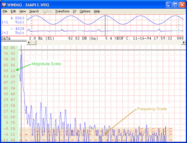
After the data window type, number of points, and input averaging (optional) selections have been made, activate the OK command button to calculate the FFT. When calculated, the following screen is displayed. This screen is composed of three basic sections; the Y-T waveform area, the analysis reporting area, and the FFT plot area.
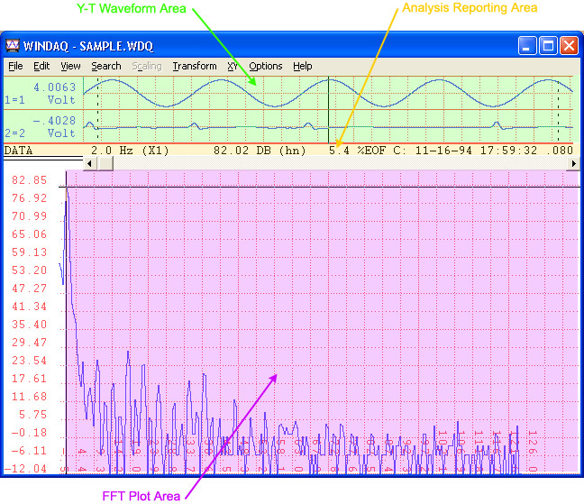
An example screen showing how the FFT screen is divided.
The Y-T waveform area is divided into two windows (window 1 and window 2). Window 1 displays the waveform from which the transform was derived. Window 2 initially displays the waveform it contained before the transform was invoked, but is used as the target window for subsequent IFTs if this feature is activated. The waveforms contained in both windows may be manipulated by using the same functions available in the Y-T mode of WinDaq Waveform Browser software while a power spectrum is displayed.
Following the transform, three cursors will appear in the Y-T waveform area to show the portion of the waveform that was used to generate the power spectrum.
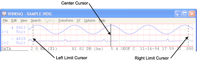
The center cursor is automatically placed in the center of the screen to indicate the center of the FFT. The left cursor indicates the left limit of the FFT range, which is 512 pixels away from the center on a 1024 x 768 display. The right cursor indicates the right limit of the FFT range, which is 511 pixels to the right of the center cursor on a 1024 x 768 display. The actual data used in the FFT calculation is the raw data contained between the two limit cursors. Assuming that a compression factor of one (1) was enabled at the time the FFT was activated, and a full screen (not resized) display is used, a 1024 point FFT will be generated.
The analysis reporting area performs a dual role. When manipulating the waveforms in the Y-T area, the analysis reporting area contains information about the waveforms in this area just as a typical WinDaq Waveform Browser screen would. When examining the power spectrum in the FFT plot area, the analysis reporting area changes to display information about the setup conditions and the power spectrum data. This data is updated as the cross hair, displayed on the power spectrum plot, is moved. A typical display with the cross hair placed over a frequency of 6.40 Hz with a relative magnitude of -99.34 dB is shown as follows:
![]()
The (X1) and (hn) descriptors define the zoom factor and window currently applied to the spectrum. Refer to X-axis Scaling and Power Spectrum Windowing for further information related to these functions. When the analysis reporting area is displaying power spectrum data, the display can be toggled to show normal waveform information by clicking in the left/right annotation area of either waveform displayed in the Y-T area. Similarly, when the analysis reporting area is displaying waveform information, the display can be toggled to show power spectrum data by clicking anywhere in the FFT plot area.
The FFT plot area contains the actual plot of the power spectrum. Examining the power spectrum is possible through use of a cross hair which may be moved anywhere on the plot. When the FFT is plotted, the origin of the cross hair is placed at the strongest frequency component of the waveform by default. The position of this cross hair is displayed in the analysis reporting area in terms of its frequency and magnitude as described above.
The vertical crosshair can be moved to display a specific frequency value in the analysis reporting area. Clicking the left mouse button anywhere in the FFT plot area allows you to position the vertical cross hair at the mouse pointer position. Dragging anywhere in the FFT plot area with the left mouse button held down allows you to drag the vertical cross hair anywhere on the plot. When dragged the horizontal crosshair follows the plot, and the analysis reporting area updates to reveal current values. After releasing the left button, SHIFT+F4 will rescale the power spectrum plot to place the horizontal crosshair at the top of the FFT plot area and use it as the 0dB reference. This rescale can be undone by dragging the left mouse button in the left magnitude scale margin to position the horizontal cross hair at the very bottom of the FFT plot area, then by pressing SHIFT+F4 again.
The horizontal crosshair can be moved to display a specific decibel or magnitude value in the analysis reporting area. Clicking the left mouse button anywhere in the left magnitude scale margin allows you to position the horizontal cross hair at the mouse pointer position. Dragging anywhere in the left magnitude scale margin with the left mouse button held down allows you to drag the horizontal cross hair anywhere on the plot and simultaneously update the decibel or magnitude value in the analysis reporting area. After releasing the left button, SHIFT+F4 will rescale the power spectrum plot to place the horizontal crosshair at the top of the FFT plot area and use it as the 0dB reference. This rescale can be undone by dragging the left mouse button in the left magnitude scale margin to position the horizontal cross hair at the very bottom of the FFT plot area, then by pressing SHIFT+F4 again.
Grid lines and axis annotation are also available to aid waveform analysis. Grid lines can be toggled on and off in the same manner as described in the Screen Grid Pattern Control function. When displayed, the X-axis of the plot represents the frequency axis of the power spectrum with the scale displayed at the bottom of the screen. The Y-axis represents the magnitude axis of the power spectrum with the scale displayed at the left edge of the screen. The magnitude axis (Y-axis) is always displayed when a transform is performed, however the frequency axis (X-axis) can be toggled on and off by selecting the Limit & Frequency Display command from the Options menu.
See also Split Screen Operations.